Chap3-神经网络
Notes
结构:输入层-中间层(隐藏层)-输出层
激活函数:
\[h(x) = \begin{cases} 0 & (x \leq 0) \\ 1 & (x > 0)\end{cases}\]
可以将感知机改写成:
\[a = b + w_1x_1+ w_2x_2, \quad y = h(a)\]
将感知机的激活函数从阶跃变成连续函数,就进入了神经网络.
如:sigmoid函数
\[h(x) = \dfrac{1}{1+ \exp(-x)}\]
阶跃函数的numpy下python实现:
def step_function(x):       # x = np.array([-1.0, 1.0, 2.9])
    y = x > 0              # 对每个元素进行判断,生成bool数组np.array([False, True, True])
    return y.astype(np.int) # 类型转换,把 False 变成 0,True 变成 1, 返回 np.array([0, 1, 1])
进一步地,
绘图:
import numpy as np
import matplotlib.pylab as plt
def step_function(x):
    return np.array(x > 0, dtype = np.int)
x = np.arange(-5.0, 5.0, 0.1)
y = step_function(x)
plt.plot(x, y)
plt.ylim(-0.1, 1.1) # y轴范围从 -0.1 到 1.1
plt.show()
ReLU (Rectified Linear Unit)函数:
\[h(x) = \begin{cases} x & (x > 0) \\ 0 & (x \leq 0)\end{cases}\]
多维数组运算:
>>> import numpy as np
>>> A = np.array([1,2,3,4])
>>> print(A)
[1 2 3 4]
>>> np.ndim(A)
1
>>> A.shape
(4,)
>>> A.shape[0]
4
ndim返回列数. shape[0]返回行数,shape[1]返回列数.
>>> B = np.array([[1,2], [3,4], [5,6]])
>>> print(B)
[[1 2]
 [3 4]
 [5 6]]
>>> np.ndim(B)
2
>>> B.shape
(3, 2)
>>> B.shape[0]
3
矩阵乘法实现:
>>> A = np.array([[1,2], [3,4]])
>>> A.shape
(2, 2)
>>> B = np.array([[5,6], [7,8]])
>>> B.shape
(2, 2)
>>> np.dot(A,B)
array([[19, 22],
       [43, 50]])
乘法成立的充分必要条件:np.ndim(A) = A.shape[1] = B.shape[0]
三层神经网络前向处理(从输入到输出)实现:
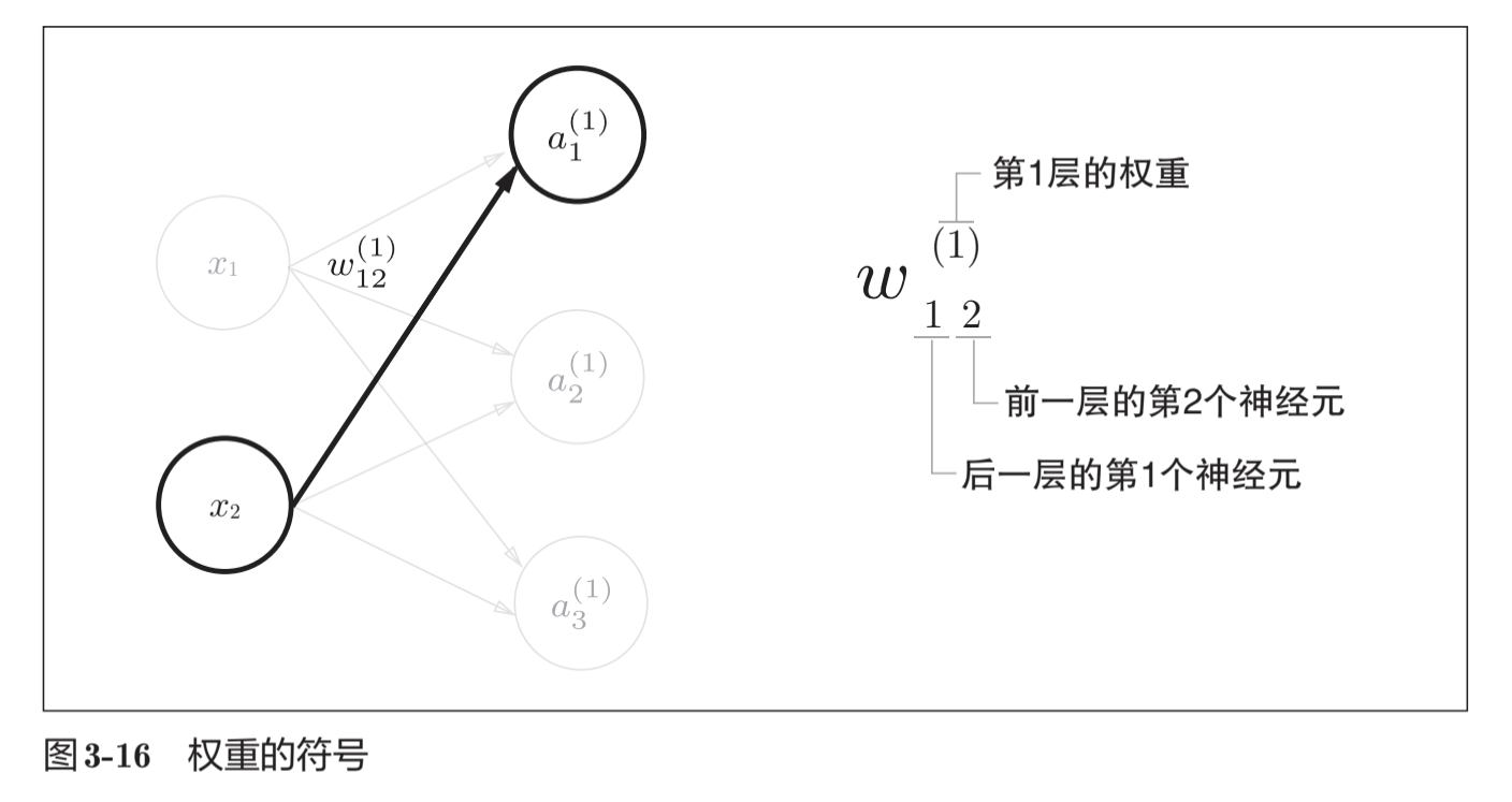
\[a_1^{(1)} = w_{11}^{(1)}x_1 + w_{12}^{(1)}x_2 + b_{1}^{(1)}\]
加权和写法:
\[A^{(1)} = XW^{(1)} + B^{(1)}\]
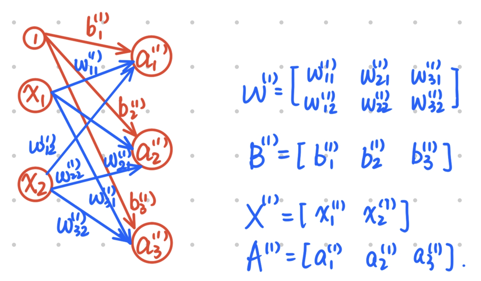
X = np.array([1.0, 0.5])
W1 = np.array([[0.1, 0.3, 0.5], [0.2, 0.4, 0.6]])
B1 = np.array([0.1, 0.2, 0.3])

A1 = np.dot(X, W1) + B1
Z1 = sigmoid(A1)

W2 = np.array([[0.1, 0.4], [0.2, 0.5], [0.3, 0.6]])
B2 = np.array([0.1, 0.2])

A2 = np.dot(Z1, W2) + B2
Z2 = sigmoid(A2)

def identity_function(x):
    return x

W3 = np.array([[0.1, 0.3], [0.2, 0.4]])
B3 = np.array([0.1, 0.2])
A3 = np.dot(Z2, W3) + B3

Y =  identity_function(A3)
在输出层的激活函数用\(\sigma\)表示,而不是\(h()\).
整理实现:
def init_network():
    network = {}
    network['W1'] = np.array([[0.1, 0.3, 0.5], [0.2, 0.4, 0.6]])
    network['B1'] = np.array([0.1, 0.2, 0.3])
    network['W2'] = np.array([[0.1, 0.4], [0.2, 0.5], [0.3, 0.6]])
    network['B2'] = np.array([0.1, 0.2])
    network['W3'] = np.array([[0.1, 0.3], [0.2, 0.4]])
    network['B3'] = np.array([0.1, 0.2])
    return network

def forward(network, x):
    W1, W2, W3 = network['W1'], network['W2'], network['W3']
    B1, B2, B3 = network['B1'], network['B2'], network['B3']

    a1 = np.dot(x, W1) + B1
    z1 = sigmoid(a1)
    a2 = np.dot(z1, W2) + B2
    z2 = sigmoid(a2)
    a3 = np.dot(z2, W3) + B3
    z3 = identity_function(a3)

    return y

network = init_network()
x = np.array([1.0,0.5])
y = forward(network, x)
print(y)
输出层可以用softmax函数来设计.
\[y_k = \dfrac{\exp(a_k)}{\sum\limits_{i = 1}^n \exp(a_i)}\]
当某些数太大的时候,会造成溢出,其改进方法是:
\[\begin{aligned} y_k = \dfrac{\exp(a_k)}{\sum\limits_{i = 1}^n \exp(a_i)} = \dfrac{C \exp(a_k)}{C \sum\limits_{i = 1}^n \exp(a_i)} \\ = \dfrac{\exp(a_k+ \log C)}{\sum\limits_{i = 1}^n \exp(a_i + \log C)} \\ = \dfrac{\exp(a_k + C')}{\sum\limits_{i = 1}^n \exp(a_i + C')}\end{aligned}\]
举例:
>>> a = np.array([1010, 1000, 990])
>>> np.exp(a) / np.sum(np.exp(a))
<stdin>:1: RuntimeWarning: overflow encountered in exp
<stdin>:1: RuntimeWarning: invalid value encountered in true_divide
array([nan, nan, nan])
>>> c = np.max(a)
>>> c
1010
>>> a = a-c
>>> np.exp(a) / np.sum(np.exp(a))
array([9.99954600e-01, 4.53978686e-05, 2.06106005e-09])
所以可以对softmax进行防溢出改进:
def softmax(a):
    c = np.max(a)
    exp_a = np.exp(a-c)
    sum_exp_a = np.sum(exp_a)
    y = exp_a / sum_exp_a

    return y