Colab 0
基础语法
Graph
G = nx.Graph()   # 无向图
print(G.is_directed())

H = nx.DiGraph() # 有向图

G.graph["Name"] = "Bar"

print(H.is_directed())
print(G.graph)
结果:
Node
重要的函数:
-
add_node,nodes(),add_nodes_from -
number_of_nodes()
G.add_node(0, feature = 5, label = 1)

node_0_attr = G.nodes[0]
print("Node 0 has the attributes {}".format(node_0_attr))

# 输出:Node 0 has the attributes {'feature': 5, 'label': 1}
查看所有节点的属性 (data=True表示显示节点相关的数据,默认data=False表示查看有哪些节点):
G.nodes(data = True)

# 输出:NodeDataView({0: {'feature': 5, 'label': 1}})

G.nodes()

# 输出:NodeView((0,))
一次性添加多个节点:
查看所有节点信息:
for n in G.nodes(data=True):
    print(node)

num_nodes = G.number_of_nodes()
print("G has {} nodes".format(num_nodes))

# 输出:
# (0, {'feature': 5, 'label': 1})
# (1, {'feature': 1, 'label': 1})
# (2, {'feature': 2, 'label': 2})
# G has 3 nodes
并且提供了可视化的方法.
调用邻居节点:
node_id = 1
for neighbor in G.neighbors(node_id):
    print("Node {} has neighbor {}".format(node_id, neighbor))

# 输出:
# Node 1 has neighbor 0
# Node 1 has neighbor 2
nx.path_graph(num_nodes)

num_nodes = 4
G = nx.DiGraph(nx.path_graph(num_nodes))
nx.draw(G, with_labels = True)

pr = nx.pagerank(G, alpha=0.8)
print(pr)

# {0: 0.17857162031103999,
# 1: 0.32142837968896,
# 2: 0.32142837968896,
# 3: 0.17857162031103999}
PyTorch Geometric Tutorial
简称PyG包,安装与使用:
依赖安装:
pip install -q torch-scatter -f https://data.pyg.org/whl/torch-2.4.0+cu121.html
pip install -q torch-sparse -f https://data.pyg.org/whl/torch-2.4.0+cu121.html
pip install -q torch-geometric
Basics
可视化函数:根据传入h的类型选择可视化方法,是张量的时候用numpy,是NetworkX图对象的时候选择spring_layout算法可视化
import torch
import networkx as nx
import matplotlib.pyplot as plt

def visualize(h, color, epoch=None, loss=None, accuracy=None):
    plt.figure(figsize=(7,7))
    plt.xticks([])
    plt.yticks([])

    if torch.is_tensor(h):
        h = h.detach().cpu().numpy() # 从计算图中分离,转为numpy
        plt.scatter(h[:, 0], h[:, 1], s = 140, c = color, cmap = "Set2") # 取前两维作为 x/y 坐标散点图
        if epoch is not None and loss is not None and accuracy['train'] is not None and accuracy['val'] is not None: # 训练信息完整的情况下,在x轴上额外标注信息
            plt.xlabel((f'Epoch: {epoch}, Loss: {loss.item():.4f} \n'
                        f'Training Accuracy: {accuracy["train"]*100:.2f}% \n'
                        f' Validation Accuracy: {accuracy["val"]*100:.2f}%'),fontsize=16)
    else:
        nx.draw_networkx(h, pos=nx.spring_layout(h, seed=42), with_labels=False,
                         node_color=color, cmap="Set2")
    plt.show()
数据集获取:通过torch_geometric.datasets来得到,此处使用KarateClub数据集.
from torch_geometric.datasets import KarateClub

dataset = KarateClub()
print(f'Dataset: {dataset}:')
print('======================')
print(f'Number of graphs: {len(dataset)}')
print(f'Number of features: {dataset.num_features}')
print(f'Number of classes: {dataset.num_classes}')

# 输出:
'''
Dataset: KarateClub():
======================
Number of graphs: 1
Number of features: 34
Number of classes: 4
'''
查看其中一组数据:
data = dataset[0]

print(data)
print('===============================================================')
print(f"Number of nodes: {data.num_nodes}")
print(f"Number of edges: {data.num_edges}")
print(f"Average node degree: {(data.num_edges) / data.num_nodes:.2f}")
print(f'Number of training nodes: {data.train_mask.sum()}')
print(f'Training node label rate: {int(data.train_mask.sum()) / data.num_nodes:.2f}')
print(f'Contains isolated nodes: {data.has_isolated_nodes()}')
print(f'Contains self-loops: {data.has_self_loops()}')
print(f'Is undirected: {data.is_undirected()}')

'''
输出:
Data(x=[34, 34], edge_index=[2, 156], y=[34], train_mask=[34])
===============================================================
Number of nodes: 34
Number of edges: 156
Average node degree: 4.59
Number of training nodes: 4
Training node label rate: 0.12
Contains isolated nodes: False
Contains self-loops: False
Is undirected: True
'''
Data
每一个PyG中的graph都是用Data对象来表示的,如:
Data(edge_index=[2,156], x=[34,34], y = [34], train_mask=[34])
print(data)

# 输出:
# print(data)
# Data(x=[34, 34], edge_index=[2, 156], y=[34], train_mask=[34])
Edge Index
我们打印edge_index:
from IPython.display import Javascript

display(Javascript('''google.colab.output.setIframeHeight(0, true, {maxHeight:300})'''))

edge_index = data.edge_index
print(edge_index.t())
这种表示一般应用在稀疏图中,称 COO format (coordinate format),区别于稠密图常用的邻接矩阵表示法.
Implementing GNN
最简单的GNN operator之一是GCN layer,在PyG中使用GCNConv来实现.
GNN希望将input graph \(G = (V, E), \forall v_i \in V, X_i^{(0)}\)是其对应特征向量,通过学习得到的函数\(f_{G}: V \times \mathbb R^{d_1} \rightarrow \mathbb R^{d_2}\)(接收单个node \(v_i\)和其特征向量,输出对应的embedding向量),从而得到有利于后续任务的节点表示结果.
取前向传播过程中的激活函数为\(f(x) = \tanh(x)\),这样可以引入非线性的分类,同时把输出限制在\((-1,1)\),适合嵌入表示.
import torch
from torch.nn import Linear # 普通全连接层,用作最终分类
from torch_geometric.nn import GCNConv # 图卷积层

class GCN(torch.nn.Module):
    def __init__(self):
        super().__init__()
        torch.manual_seed(1234) # 固定随机种子,保证可复现性
        self.conv1 = GCNConv(dataset.num_features, 4) # 34维向量压缩成4维
        self.conv2 = GCNConv(4, 4)
        self.conv3 = GCNConv(4, 2)
        self.classifier = Linear(2, dataset.num_classes)

    def forward(self, x, edge_index):
        h = self.conv1(x, edge_index)
        h = h.tanh()
        h = self.conv2(h, edge_index)
        h = h.tanh()
        h = self.conv3(h, edge_index)
        h = h.tanh()

        out = self.classifier(h)

        return out, h

model = GCN()
print(model)
输出结果:
GCN(
  (conv1): GCNConv(34, 4)
  (conv2): GCNConv(4, 4)
  (conv3): GCNConv(4, 2)
  (classifier): Linear(in_features=2, out_features=4, bias=True)
)
接着进行可视化:
model = GCN()

_, h = model(data.x, data.edge_index)
print(f"Embedding shape: {list(h.shape)}")

visualize(h, color = data.y)
Training
import time
from IPython.display import Javascript  # Restrict height of output cell.
display(Javascript('''google.colab.output.setIframeHeight(0, true, {maxHeight: 430})'''))

model = GCN()
criterion = torch.nn.CrossEntropyLoss()  # Define loss criterion.
optimizer = torch.optim.Adam(model.parameters(), lr=0.01)  # Define optimizer.

def train(data):
    optimizer.zero_grad()  # Clear gradients.
    out, h = model(data.x, data.edge_index)  # Perform a single forward pass.
    loss = criterion(out[data.train_mask], data.y[data.train_mask])  # Compute the loss solely based on the training nodes. 是核心,只用带标签的节点计算损失
    loss.backward()  # Derive gradients.
    optimizer.step()  # Update parameters based on gradients.

    accuracy = {}
    # Calculate training accuracy on our four examples
    predicted_classes = torch.argmax(out[data.train_mask], axis=1) # [0.6, 0.2, 0.7, 0.1] -> 2
    target_classes = data.y[data.train_mask]
    accuracy['train'] = torch.mean(
        torch.where(predicted_classes == target_classes, 1, 0).float())

    # Calculate validation accuracy on the whole graph
    predicted_classes = torch.argmax(out, axis=1)
    target_classes = data.y
    accuracy['val'] = torch.mean(
        torch.where(predicted_classes == target_classes, 1, 0).float()) # 评估泛化能力

    return loss, h, accuracy

for epoch in range(500):
    loss, h, accuracy = train(data)
    # Visualize the node embeddings every 10 epochs
    if epoch % 10 == 0:
        visualize(h, color=data.y, epoch=epoch, loss=loss, accuracy=accuracy)
        time.sleep(0.3)
最终的结果图(epoch = 490):
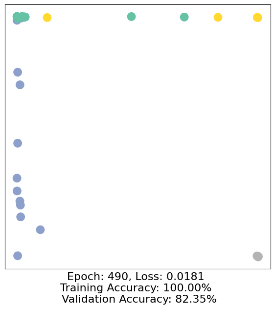
可以看出确实分成了4个社群,节点坐标是GCN学习得到的2维embedding向量.
指标上:
Epoch: 490        训练接近尾声
Loss: 0.0181      损失极低,训练集拟合很好
Training Acc: 100%  训练节点全部分对
Val Acc: 82.35%   全图有约18%节点分类错误
说明有一点过拟合了.