8.Performance Profiling

2026.7.12，原标题为 Introduction to Profiling: Latency, Throughput, and How to Measure Them

这节课贯穿始终的问题是：为什么下面的两段矩阵加法代码效率天差地别？以及，如何做到如此大的优化？

A. 0.53 GFLOP/s

for (long i = 0; i < n; i++)
  for (long j = 0; j < n; j++)
      for (long k = 0; k < n; k++)
          C[i * n + j] += A[i * n + k] * B[k * n + j];

B. 3,170 GFLOP/s，接近6000的speedup!

cblas_dgemm(CblasRowMajor, CblasNoTrans, CblasNoTrans, n, n, n,
         1.0, A, n, B, n, 0.0, C, n);

What is Performance

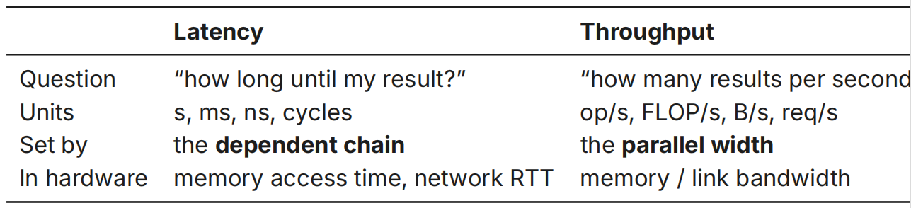
衡量一个系统的快慢有两个指标：

• Latency：一个operation花费的时间
• Throughput：单位时间内完成的操作数

举个例子，玩FPS时你希望自己每次鼠标点击的延迟能够降低到20ms，这就是Latency；整个服务器能够支持2w玩家同时在线团战，这就是Throughput.

一个耳熟能详的场景是，一辆载满了硬盘的大卡车，此时可以说它具有enormous throughput, terrible latency.

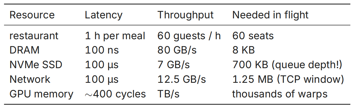
在这两个参数的基础上，要考察硬件的瞬时承载能力，我们引入了Little's Law：

\[ \text{in-flight} = \text{Throughput} \times \text{Latency} \]

这可以用一个KFC餐厅来建模理解. 假设每个顾客平均要在店里面吃1h疯狂星期四再离开，且每小时会进来60个顾客，那么所需要的椅子数自然就是

\[ 60 \text{guests}/h \times 1h = 60 \]

实际上，Little's Law几乎遍布体系结构的各个地方：

在流水线CPU中，我们做到的事就是，提升Throughput，保持Latency，从而获得了更大的in-flight. 课程中采用的AMX架构也做到了这件事：当一个FMA开始执行时，对下一次iteration的装载已经开始：

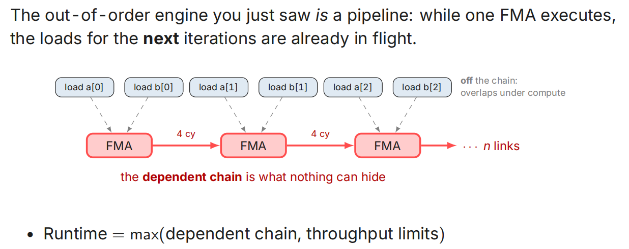
Dependency Chain (依赖链)是不会撒谎的，会将完整的运行过程揭露出来.

接下来我们考察以下例子：

for (long i = 0; i < n; i++) s += a[i] * b[i]; // one chain

for (long i = 0; i < n; i += 8) { // eight chains
    s0 += a[i] * b[i]; s1 += a[i + 1] * b[i + 1];
    /* ... */ s7 += a[i + 7] * b[i + 7];
}

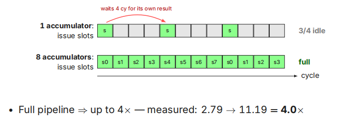
上下2种的编译有非常大的速度差距：

$ gcc {flags} dot1v8.c                  1 acc 8 accs
    -O2                                 2.79 8.48
    -O3 -march=native                    2.79 11.19
    -O2 -ffast-math                      5.56 9.49
    -O3 -march=native -ffast-math         11.13 17.88

究其原因，FMA单元是一个流水线，Latency = 4cycles，但是每个cycle可以进行一个新的独立op：

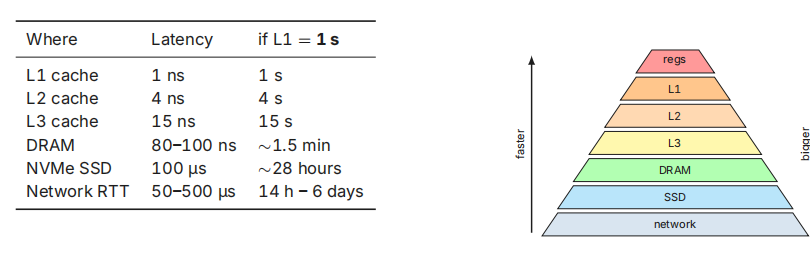
我们已经学习过，层次图上越往上，体积越小且latency越少：

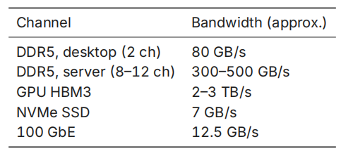
而如果从Bandwidth角度来看Memory数据：

Measuring the Machine

Profiling the Program