CS188-Introduction to Artifitial Intelligence[2025_Spring-UC Berkley]
课程网址:CS 188 Spring 2025 Introduction to Artificial Intelligence at UC Berkeley
Notes地址:Introduction to Artificial Intelligence
这是课程网站存档,虽然不会立刻失效,但是还是要加紧学习,毕竟AI技术迭代太快了。
课程Calendar


Week1-Intro & Uninformed Search
对应的是FDS课程的Depth-First Search, Breadth-First Search, Uniform-Cost Search内容.
-
Depth-First Search:
last in first out, selects the deepest frontier node from the start node for expansion.
-
Breadth-First Search:
first in first out, selects the shallowest frontier node from the start node for expansion.
It prioritizes the expansion of shallow nodes. Therefore, the search always returns a path with the smallest number of edges.
-
Uniform Cost Search:
always selects the lowest cost frontier node from the start node for expansion.
It prioritizes the expansion of paths with low costs in the fringe. Therefore, the search always returns a path with the lowest cost.
The general pseudocode for tree/graph search:
function TREE-SEARCH(problem, frontier) return a solution or failure
    frontier ← INSERT(MAKE-NODE(INITIAL-STATE[problem]), frontier)
    while not IS-EMPTY(frontier) do
        node ← POP(frontier)
        if problem.IS-GOAL(node.STATE) then return node
        for each child-node in EXPAND(problem, node) do
            add child-node to frontier
    return failure
The expand function:
function EXPAND(problem, node) yields nodes
    s ← node.STATE
    for each action in problem.ACTIONS(s) do
        s' ← problem.RESULT(s, action)
        yield NODE(STATE=s', PARENT=node, ACTION=action)
Annalysis:
We suppose that there are $\textcolor{red}{b}$ nodes in the second layer, and if the depth +1, the number of nodes $\times b$.
The goal is on the $\textcolor{red}{s}$ tier, and and maximum depth is $\textcolor{red}{m}$.
| DFS | BFS | UCS | |
|---|---|---|---|
| Completeness(完备性) | × | √ | √ |
| Optimality(最优性) | × | × | √ |
| Time Complexity | $O(b^m)$ | $O(b^s)$ | $O(b^{\frac{C^*}{\epsilon}})$ |
| Space Complexity | $O(bm)$ | $O(b^s)$ | $O(b^{\frac{C^*}{\epsilon}})$ |
In UCS, we define the optimal path cost as $\textcolor{red}{C^∗}$ and the minimal cost between two nodes in the state space graph as $\textcolor{red}{\epsilon}$.
Three strategies above are fundamentally the same - differing only in expansion strategy, so they share the pseudocode above.
TIP
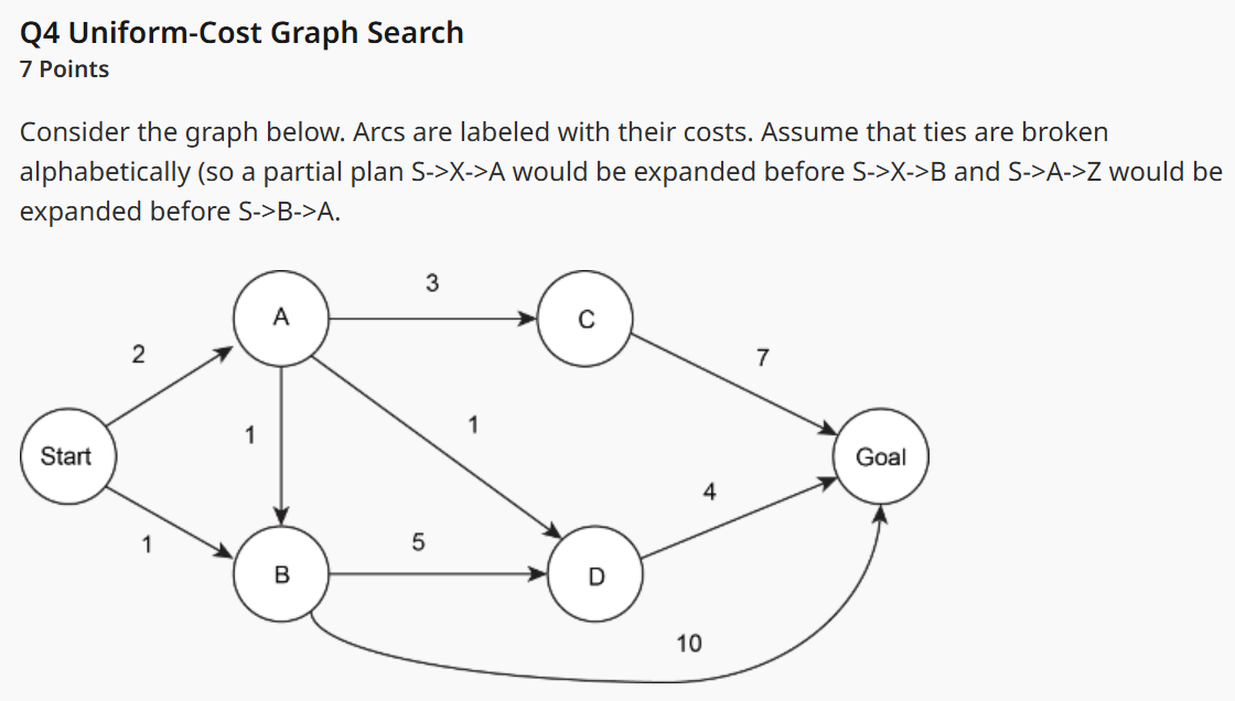
UCS eg.
step 1 2 3 4 5 6 7 expand S S-B S-A S-A-D S-A-C pop S-B-D S-A-D-G fringe (S-A, 2), (S-B, 1) (S-A, 2), (S-B-D, 6), (S-B-G, 11) (S-B-D, 6), (S-B-G, 11), (S-A-D, 3), (S-A-C, 5) (S-B-D, 6), (S-B-G, 11), (S-A-C, 5), (S-A-D-G, 7) (S-B-D, 6), (S-B-G, 11), (S-A-D-G, 7), (S-A-C-G, 12) (S-B-G, 11), (S-A-D-G, 7), (S-A-C-G, 12) Nothing to fringe closed set S S,B S,B,A S,B,A,D S,B,A,D,C S, B, A, D, C S, B, A, D, C, G Return: Start-A-D-Goal